L-systems explorer
Table of Contents
Overview
L-systems were originally introduced in 1968 by Aristid Lindenmayer as a mathematical model for the development of cellular organism and plants. They consist of a set of production rules that are used to replace each symbol inside a string by some new string. The strings produced by the rules are then interpreted as instructions for a turtle graphics program which produces a graphical representation of the model (which does not necessarily have to be very plant-like).
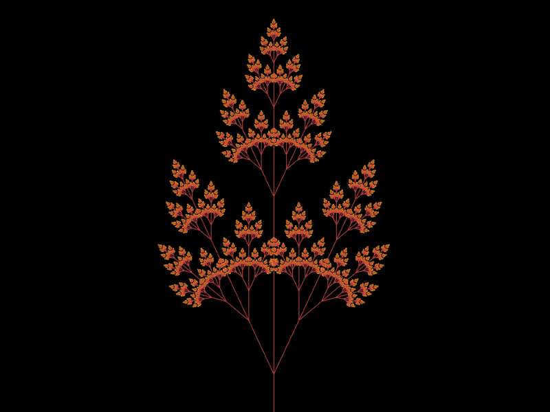
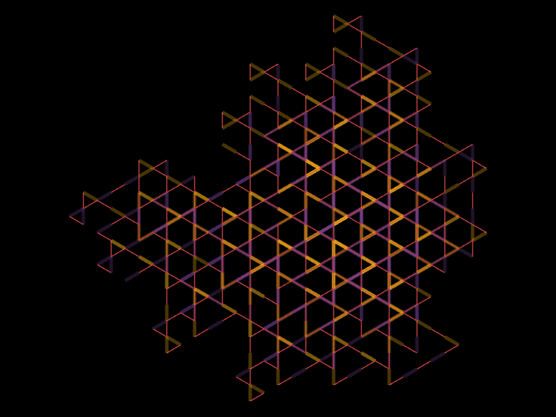
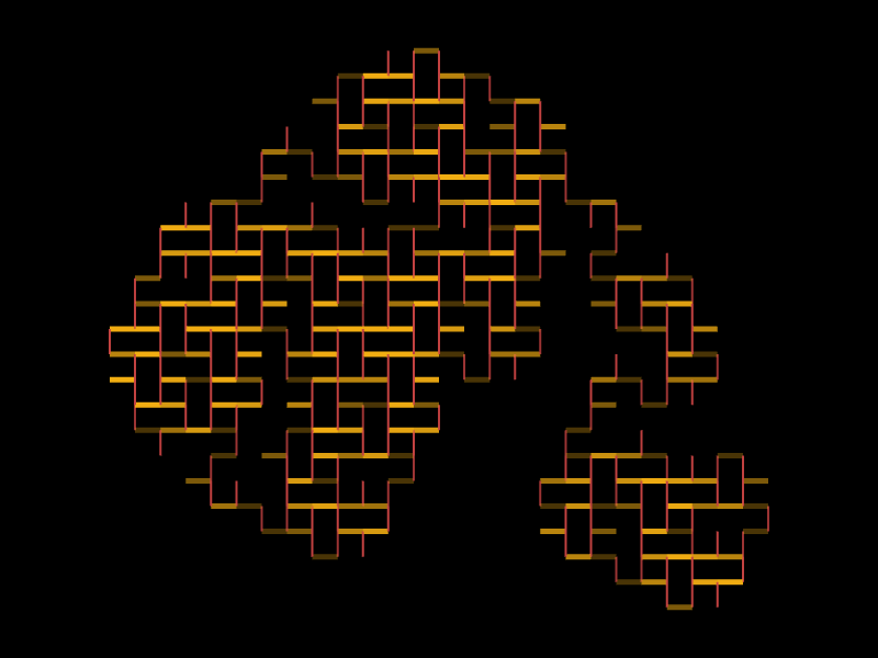
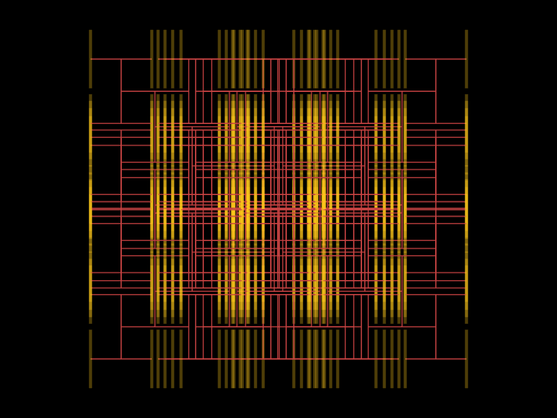
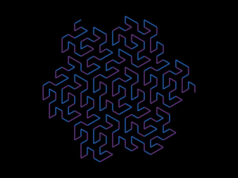
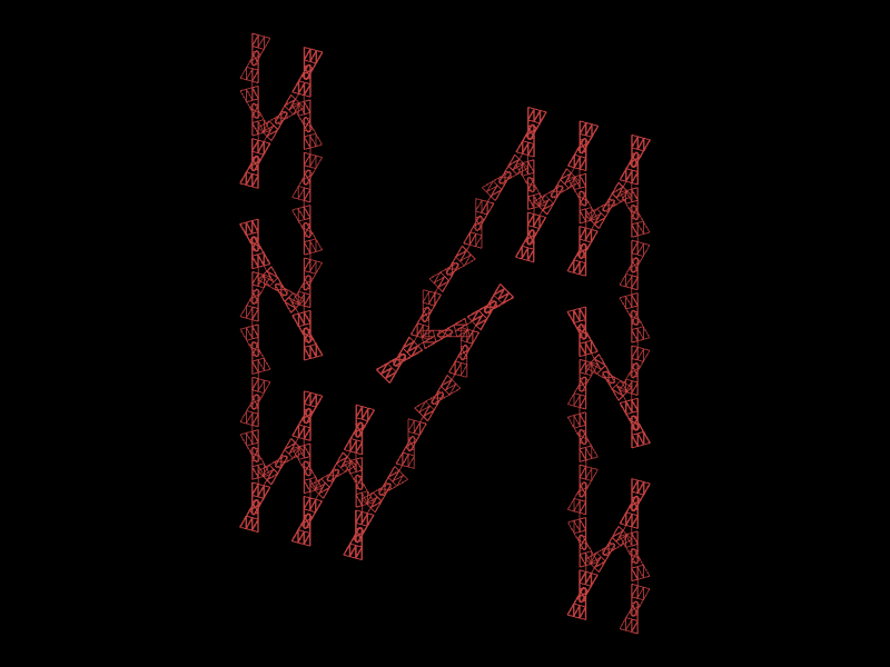
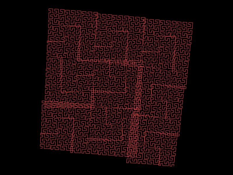
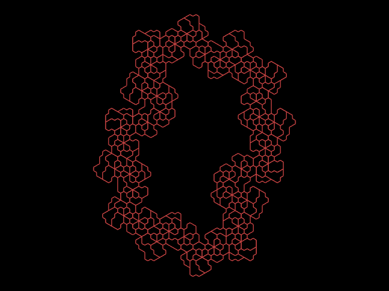
Below I made a tool to draw the graphical representation of some L-systems (taken from the book The Algorithmic Beauty of Plants). Here are some pictures produced by it:
The tool itself is far from complete and has many rough edges.
You can select from some systems defined in the book The Algorithmic Beauty of Plants (the number refer to the figures in that book), modify them or define your own set of production rules.
To render the system press Shift + Enter or the "render" button.
There is also the option to enable live update when the parameters change.
Some background and explanations about the different parameters can be found below.
- length (number of symbols)
- -
- max. stack height
- -
- derivation
- -
- fill position buffer
- -
- render
- -
L-systems and turtle graphics
An L-system consists of a set of symbols \(S\), a non-empty word \(\omega \in S^+\) called the axiom and a finite set of production rules \(P \subset S \times S^\star\). Here \(S^\star\) and \(S^+\) denote the sets of all and all non-empty words over \(S\) respectively.
A production \(p \in P\) is a tuple \((s, w)\) with \(s \in S\) a symbol and \(w \in S^\star\) as word and is usually written as \(s \to w\). There is at least one production for every symbol \(s \in S\); if no production is given explicitly it is assumed to be the identity \(s \to s\).
Given a word \(\omega = s_1 \ldots s_m\) we can derive a new word \(\omega' = w_1 \ldots w_m\) by simultaneously replacing all symbols \(s_i\) according to a production rule \(s_i \to w_i\). Iterating this process we obtain a sequence of words \(\omega, \omega', \omega'', \ldots, \omega^{(i)}, \ldots\). We call \(i\) the level of the word \(\omega^{(i)}\) obtained after \(i\) iterations.
Here is a simple example: Let \(S = \{F, +\}\) and let the axiom \(\omega = F\) and the only non-trivial production be given by
\begin{align} p: F \to F+F. \end{align}From this system we obtain the following sequence of words:
\begin{align} \begin{split} \omega &: \quad F \\ \omega^{(1)} &: \quad F+F \\ \omega^{(2)} &: \quad F+F+F+F \\ \omega^{(3)} &: \quad F+F+F+F+F+F+F+F \\ \omega^{(4)} &: \quad \cdots \end{split} \end{align}A graphical representation of such words can be derived by interpreting them as instructions for a turtle graphics program. The idea is to place a turtle (with a pen) at some position \((x, y)\) in the plane, heading in some direction \(\alpha\). The various symbols in the alphabet \(S\) are interpreted as instructions for the turtle to move around and draw lines on the plane.
For example, the symbol \(F\) instructs the turtle to move forward by some fixed amount while drawing a line. The symbol \(+\) represents a rotation to the right by some fixed angle (i.e. a change in heading). With an angle of 45 degrees, the word \(\omega^{(3)}\) from above would have the following interpretation:
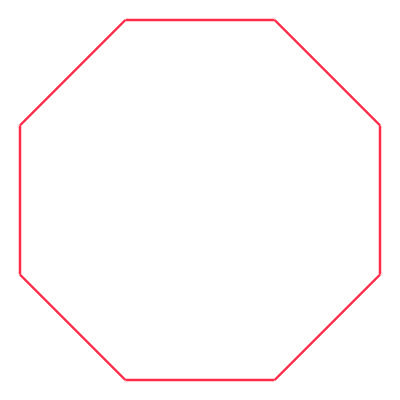
Figure 1: Turtle interpretation of \(F+F+F+F+F+F+F+F\).
There are now some ways to extend the instruction set to allow the turtle to draw more complex shapes:
The current state of the turtle (consisting of its position, orientation and line width) can be pushed onto a stack with the symbol \([\). The symbol \(]\) pops a state from this stack and replaces the current turtle state by it.
Moreover, the instructions may take numerical parameters. For the drawing and moving commands a parameter \(s\) is interpreted as a step size. The symbol \(F(4.0)\) for instance instructs the turtle to move forward by four units. For the rotation commands a parameter \(a\) is interpreted as an angle and overrides the global angle parameter.
The right-hand side of a production rule can involve mathematical expressions of the parameters, e.g.
\begin{align} F(s, a) \to F(s, a / 2) +(a) F(s, a / 2). \label{eq:example-parameters} \end{align}The parameter \(a\) for the rotation symbol is interpreted as an angle. Starting with the axiom \(F(1.0, 90)\), the word \(\omega^{(3)}\) looks as follows:
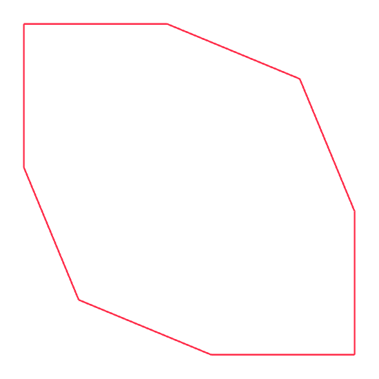
Figure 2: Turtle interpretation of \(\omega^{(3)}\) derived from axiom \(F(1.0, 90)\) with rule \eqref{eq:example-parameters}
Finally, the turtle is allowed to move in three rather than just two dimensions. To fully specify the orientation we therefore need three axes: the heading, an axis pointing to the left and another one pointing up from the point of view of the turtle. We also allow rotations around each of these axes.
The available symbols are summarized in the following table.
| Symbol(s) | Interpretation |
|---|---|
| \(A(s), \ldots, Z(s)\) | Move step size \(s\) while drawing a line |
| \(f(s)\) | Move step size \(s\) without drawing a line |
| \([\), \(]\) | Push to / pop from turtle stack |
| \(+(\alpha)\), \(-(\alpha)\) | Rotate around "up" axis by angle \(\pm \alpha\) |
| \(\&(\alpha)\), \(\wedge(\alpha)\) | Rotate around "left" axis by angle \(\pm \alpha\) |
| \(<(\alpha)\), \(>(\alpha)\) | Rotate around "heading" axis by angle \(\pm \alpha\) |
| \(!(s)\) | Set line width to \(s\) |
There is also the option to set a tropism vector \(T\). After every drawing step the turtle rotates towards \(T\) by an angle proportional to \(|H \times T|\) where \(H\) is the current heading. This introduces a preferred direction as for instance caused by gravity. Unfortunately I did not implement this correctly and the turtle simply always rotates around the local "left" axis for now. It can however still be used to introduce some interesting graphical effects into the picture.
Implementation notes
The parsing of the rule string is a complete mess and I should have put more work into making it better. The parameter expressions that may occur on the right-hand side of a production rule are converted to Reverse Polish Notation and stored for each symbol. In the derivation step of the next word in sequence these expressions are evaluated and only their value is kept.
Initially, a word of symbols was converted to its graphical representation by directly drawing on a canvas with the CanvasRenderingContext2D interface. This turned out to be quite slow for longer words and I decided to use the WebGL API instead. The drawing step now creates a buffer containing the end points of line segments as well as their width and color. This data is passed to a vertex shader where an instance of the same basic segment is drawn in the right location and scaled appropriately.
For long words the derivation and drawing can still take quite some time. On my laptop (from 2018), calculating \(\omega^{(12)}\) (~3.1 million symbols) for the system "Plant like (ABP 1.24e)" takes a bit under 2 seconds. Most of the time (~1.2 s) is spent in the derivation part, followed by the construction of the buffer with the line segment end points (~0.7s). The actual rendering is comparatively fast (~60 ms).
The code can be found here (sourcehut) and here (GitHub).
References
- Aristid Lindenmayer: Mathematical models for cellular interactions in development II. Simple and branching filaments with two-sided inputs
- Przemyslaw Prusinkiewicz, Aristid Lindenmayer: The Algorithmic Beauty of Plants